Maximum Likelihood Estimation and Duality in Optimization
Duality and Lagrangian Duality
duality states that a mathematical optimization problem can be subjected to an equality, and an inequality constraint in the way that:
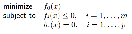
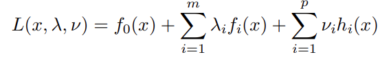
Now, Lagrangian duality states that there exists lambda, a multiplier with which:
Now, keep this in mind. Here’s what we’re going to explain in this post:
There exists a duality between Maximum Entropy and Likelihood.
Therefore:
A logistic regression model can be optimized using Maximum Likelihood.
Why? Because a logistic regressor is simply a binary Maxent model.
Discimination, Generation, and Likelihood
We have a set of features X and a set of targets y which are distributed according to an unkown distribution. We wish to estimate the conditional probability P(y|X), in other words, create a probabilistic ML model based on these data. There are two approaches.
- Discriminative approach: We use tools from learning theory ot compute a hypthesis that models the conditional probability
P(y|X)up to a small error. - Generative approach: We estimate the probability distribution
P(X|y)separately for every y. For instance y could represent the attribute gender and x could represent the attirbute height. In this case, according to Bayes’ rule:

Maximum Likelihood
Imagine our goal is to find distribution D of discrete data X. To motivate this notion, suppose D is distributed according to one out of two possible density funcqtions q1 and q2. If you’re wondering what a density function is, a Probability Density Function is a function that takes distribution from continuous space to discrete space. On the other hand, a Probability Mass Function takes a discrete distribution to continouous space.
Now, intuitively, if we observe that q1(xi) is typicalled much larger than q2(xi), we will tend to conclude that D is distributed according to q1.
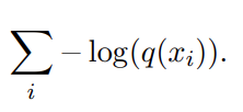
In general, we consider a sent of density functions Q. For q being a member of Q we have:
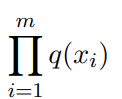
This is what we call likelihood of X under q. Notice, if Xs are independent — as in, realization of one does not affect the realization of the other — likelihood is the same as probability.
Now, logarithm has this quality which makes it monotonically increasing. This is the quality that was used in the old logarithm tables which people used to multiply large numbers before the advent of calculators. So we have:
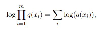
Maximizing this function is equivalent to minimizing it. So think of this as a loss function:
And thereby we introduce the true risk of q as:
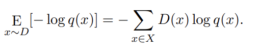
And yes, that is entropy you see besides the Sigma. Relative entropy, to be exact. This is what we call cross entropy, except with two functions — one distribution — instead of a value and a function, like in entropy. We can expand this equation like this:
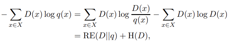
Where RE denotes relative entropy and H is normal Shannon entropy.
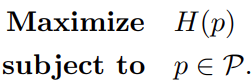
Maximum Entropy
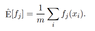
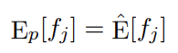
Another way of approaching the the above problem is to use the method of maximum entropy. Here, we start with the fact that we can approximate the true expected value  of each feature fj by its empirical average taken over the gien samples. In other words:
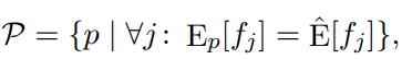
This leads to the idea of finding a distribution p which satisifes the constraint:
Now, we calculate its distance from uniform distribution by calculating the relative entropy in a way which:
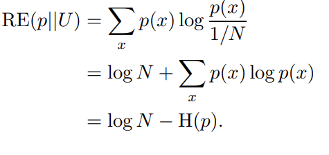
Since logarithn of N is just a constant, we can write maximum entropy as a dual problem:
Where:
Duality betwee Maxent and Likelihood
We finally arrive at this theorem:
Let q* be a probability distribution. Then, the following are equivalent:
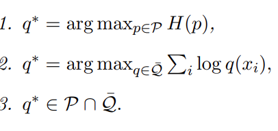
And there we are! The relationship between these two explained.